Exponential Smoothing: A Guide to Getting Started

By Community
updated March 23, 2026 Developer

Exponential smoothing is a time series forecasting method that uses an exponentially weighted average of past observations to predict future values. In other words, it assigns greater weight to recent observations than to older ones, allowing the forecast to adapt to changing data trends.

In this post, we’ll look at the basics of exponential smoothing, including how it works, its types, and how to implement it in Python.

What is exponential smoothing?

Exponential smoothing forecasts time series data by smoothing out fluctuations in the data. The technique was first introduced by Robert Goodell Brown in 1956 and then further developed by Charles Holt in 1957. It has since become one of the most widely used methods for forecasting.

The basic idea behind exponential smoothing is to give more weight to recent observations by assigning weights to each observation that decrease exponentially with age. Weights are then used to calculate a weighted moving average of the data, which is used to forecast the next period.

Exponential smoothing assumes that future values of a time series are a function of its past values. The method works well when the time series has a trend and/or a seasonal component, but it can also be used for stationary data (i.e., without trend or seasonality).

Types of exponential smoothing

There are several types of exponential smoothing methods, each with its own formulae and assumptions. The most commonly used methods include:

1. Simple Exponential Smoothing

Simple exponential smoothing (SES), also known as single exponential smoothing, is its simplest form. It assumes that the time series has no trend or seasonality.

The forecast for the next period is based on the weighted average of the previous observation and the forecast for the current period.

The formula for simple exponential smoothing is:

s_(t) = αx_(t) + (1-α)s_t-1

where

• s_(t) is the smoothed value at time t,
• x_(t) is the observed value at time t,
• s_t-1 is the previous smoothed statistic, and
• α is the smoothing parameter between 0 and 1.

The smoothing parameter α controls the weight given to the current observation and the previous forecast.

A high value of α gives more weight to the current observation, while a low value of α gives more weight to the previous forecast.

2. Holt’s Linear Exponential Smoothing

Holt’s linear exponential smoothing, also known as double exponential smoothing, is used to forecast time series data that has a linear trend but no seasonal pattern. This method uses two smoothing parameters: α for the level (the intercept) and β for the trend.

The formulas for double exponential smoothing are:

s_t = αx_t + (1 – α)(s_t-1 + b_t-1)

β_t = β(s_t – s_t-1) + (1 – β)b_t-1

where

• bt is the slope and best estimate of the trend at time t,
• α is the smoothing parameter of data (0 < α < 1), and
• β is the smoothing parameter for the trend (0 < β < 1).

Holt’s method is more accurate than SES for time series data with a trend, but it doesn’t work well for time series data with a seasonal component.

3. Holt-Winters’ Exponential Smoothing

Holt-Winters’ exponential smoothing, also referred to as triple exponential smoothing, is used to forecast time series data with both a trend and a seasonal component. It uses three smoothing parameters: α for the level (the intercept), β for the trend, and γ for the seasonal component.

The triple exponential smoothing formulas are given by:

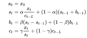
where:

• s_t = smoothed statistic; it’s the simple weighted average of current observation Y_t
• s_t-1 = previous smoothed statistic
• α = smoothing factor of data (0 < α < 1)
• t = time period
• b_t = best estimate of a trend at time t
• β = trend smoothing factor (0 < β <1)
• c_t = seasonal component at time t
• γ = seasonal smoothing parameter (0 < γ < 1)

Holt-Winters’ method is the most accurate of the three methods, but it’s also the most complex, requiring more data and computation than the other methods.

When to use exponential smoothing

Exponential smoothing is most useful for time series data that has a consistent trend, seasonality, and random fluctuations.

It’s particularly useful for short to medium-term forecasting of business metrics such as sales, revenue, and customer traffic. It’s also useful for monitoring and predicting seasonal changes in industries such as tourism, agriculture, and energy.

Here are some other common situations where exponential smoothing can be useful:

• Time series forecasting — One of the most common applications of exponential smoothing is in time series forecasting. If you have historical data for a particular variable over time, such as sales or website traffic, you can use exponential smoothing to forecast the future values of that variable.

• Inventory management — Exponential smoothing can be used to forecast demand for products or services, which can be helpful in inventory management. By forecasting demand, businesses can make sure they have enough inventory on hand to meet customer needs without overstocking.

• Finance — It can be used in finance to forecast stock prices, interest rates, and other financial variables. This can be helpful for investors who are trying to make informed decisions about buying and selling stocks or other financial instruments.

• Marketing — It’s also used to forecast the effectiveness of marketing campaigns. By tracking past campaign results and using exponential smoothing to forecast future performance, marketers can optimize their campaigns to achieve the best possible results.

Why is exponential smoothing popular?

Exponential smoothing is among the most widely used time series forecasting methods due to its simplicity and effectiveness.

Unlike other methods, exponential smoothing can adapt to changes in data trends. It also provides accurate predictions by assigning different weights to different time periods based on their importance.

Exponential smoothing is computationally efficient, making it ideal for large datasets. Additionally, it’s widely used in business forecasting, providing accurate, reliable forecasts across a range of applications, including demand, sales, and financial forecasting.

How to perform exponential smoothing

Performing exponential smoothing begins with understanding your data’s structure.

First, examine your time series to identify whether it contains trends, seasonality, or neither. This analysis will guide you in selecting the right exponential smoothing method: SES works best for stationary data, Holt’s method handles data with trends, and Holt-Winters’ method addresses both trends and seasonal patterns.

Once you’ve chosen your method, the implementation is straightforward. Modern statistical software and libraries can automatically optimize the smoothing parameters (α, β, and γ) by finding values that minimize forecast errors.

After fitting the model to your historical data, you’ll have a trained forecasting tool ready to generate predictions for future time periods.

Now, let’s put this into practice by implementing exponential smoothing using Python, one of the most popular tools for time series analysis.

Exponential smoothing in Python

Python has several libraries for exponential smoothing, including Pandas, Statsmodels, and Prophet. These libraries provide various functions and methods for implementing different types of exponential smoothing methods.

The Dataset

For this example, we’ll use the AirPassengers dataset, a time series dataset that contains the monthly number of airline passengers from 1949 to 1960. You can download the dataset from this link.

Setting Up the Environment

To get started, we need to set up our environment. We’ll be using Python 3, so make sure it’s installed. Alternatively, you can use Google Colab and go straight to importing the libraries.

Next, install these libraries using pip:

pip install pandas matplotlib statsmodels

Once you’ve installed the necessary libraries, you can import them into your Python script:

import pandas as pd
import matplotlib.pyplot as plt
from statsmodels.tsa.api import SimpleExpSmoothing

Loading the Data

After setting up the environment, we can load the AirPassengers dataset into a pandas DataFrame using the read_csv function:

data = pd.read_csv('airline-passengers.csv', parse_dates=['Month'], index_col='Month')

We can then inspect the first few rows of the DataFrame using the head function:

print(data.head())

This will output:

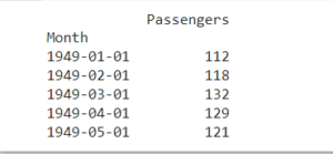
Visualizing the Data

Before we apply simple exponential smoothing to the data, let’s visualize it to get a better understanding of its properties. We can use the plot function of pandas to create a line plot of the data:

plt.plot(data)
plt.xlabel('Year')
plt.ylabel('Number of Passengers')
plt.show()

This will produce a plot of the number of passengers over time:

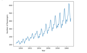
We can see that the number of passengers appears to be increasing, with some seasonality as well.

Performing SES

Now that we’ve loaded and visualized the data, we can perform simple exponential smoothing using the SimpleExpSmoothing function from the statsmodels library. Then, we’ll create an instance of the SimpleExpSmoothing class, passing in the data as an argument, and then fit the model to the data using the fit method:

model = SimpleExpSmoothing(data)
model_fit = model.fit(optimized=True)
print(model_fit.summary())

This will calculate the smoothing parameters and fit the model to the data. The optimized=True parameter allows the model to find the best smoothing parameter (α) for your data.

Making Predictions

Finally, we can use the forecast method to predict future values of the time series, where the argument specifies the number of periods to forecast.

forecast = model_fit.forecast(6)
print(forecast)

This will produce a forecast for the next six months:

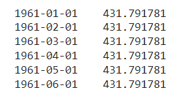
Based on the forecast, we can assume that over the next six months, there will be approximately 432 airline passengers.

Wrapping up

Exponential smoothing is a powerful method for time series forecasting that allows for accurate predictions of future values based on past observations. It’s a simple, efficient method that can be used for a wide range of time series data.

In this post, we provided a beginner’s guide to exponential smoothing, explaining the basics of the method, its types, and how to use it for forecasting. However, there are more advanced techniques and approaches to discover beyond the scope of this post.

If you’re interested in learning more, be sure to check out this Python time series forecasting tutorial. It’s a great resource that can help you deepen your understanding of this topic and take your forecasting skills to the next level with InfluxDB.

Exponential smoothing FAQs

This post was written by Israel Oyetunji. Israel is a frontend developer with a knack for creating engaging UI and interactive experiences. He has proven experience developing consumer-focused websites using HTML, CSS, JavaScript, ReactJS, SASS, and relevant technologies. He loves writing about tech and creating how-to tutorials for developers.