Anomaly Detection with Median Absolute Deviation

By Anais Dotis-Georgiou / Product, Use Cases, Developer
Jul 07, 2020

When you want to spot containers, virtual machines (VMs), servers, or sensors that are behaving differently from others, you can use the Median Absolute Deviation (MAD) algorithm to identify when a time series is “deviating from the pack”. In this tutorial, we’ll identify anomalous hosts using mad() — the Flux implementation of MAD — from a Third Party Flux Package called anaisdg/anomalydetection. We’ll find out which series is anomalous among these time series:

This dataset bears similarity to disk IO on a Linux KerneI. However, I generated this collection of time series data because I wanted to showcase the power of MAD. We are able to detect an anomalous “host” easily with mad(), even though the anomalous series isn’t immediately or easily apparent upon visual inspection.

The monetary value of anomaly detection

DevOps Monitoring enables your organization to measure key performance indicators that are mission-critical to upholding your Service Level Agreements (SLAs). Ideally, Site Reliability Engineers (SREs) use Devops Monitoring to solve operation problems, increase reliability, and guide infrastructure design efforts. Anomaly Detection algorithms like MAD enable SRE’s to identify unhealthy containers, VMs, or servers quickly. The sooner SRE’s are able to spot suspicious behaviour, the faster they are able to diagnose and remedy infrastructure problems. Root cause analysis is a highly complicated type of iterative problem solving. It involves asking deep questions and employing the Five Why’s Method. Finding the problem is just the beginning, solving operation problems can be even more challenging and require a lot of creativity. While Artificial Intelligence isn’t advanced enough to autonomously perform root cause analysis and solve infrastructure problems, anomaly detection still has value. Anomaly detection guides site reliability engineers (SREs) and sysadmins down the right path to reduce the incident resolution time or mean time to resolution (MTTR). Reduction in MTTR enables companies to honor their Service Level Objectives (SLOs), provides a good user experience, and encourages contract renewals. By allowing you to write user defined functions and incorporate custom anomaly detection algorithms, Flux provides this value. InfluxDB v2 alerts and notifications enable SREs to respond to anomalies in real-time.

How Median Absolute Deviation algorithm works

The MAD algorithm is commonly used for this type of anomaly detection because it’s highly effective and efficient. The median, or “middle” value, of all the time series at one point in time describes normal behavior for all of the time series at that timestamp. Large deviations from each individual time series and the median indicate that a series is anomalous.

The description above is a simplified overview of how the algorithm works. In actuality, a point  is flagged as anomalous by the following formula:

  (1)

where,

is your point at    (2)

is your anomalous point.  (3)

is the sample median or simply the middle value in the batch of points across series.  (4)

is a user-defined cut-off, usually 2.5 or 3.0  (4)

and is the median absolute deviation.  (5)

where,  =1.4826 is a scale factor which assumes normally distributed data.

If math isn’t your favorite subject, this algorithm might look complicated, but it’s actually really simple. Let’s break down what is actually happening with a numerical example.

Numerical example of Median Absolute Deviation

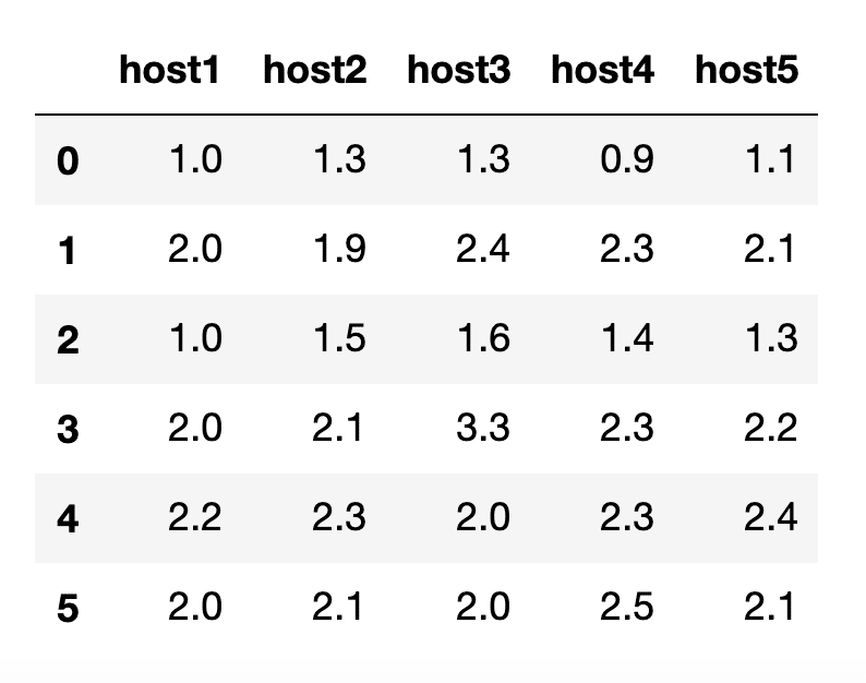
In this example, we’ll take a look at some data from different hosts. Our data looks like this with a graph (right) and table view (left):

Remember, MAD flags points as anomalous that have a large deviation from the median. Therefore the green line, host3, clearly has an anomaly at time point 3. Let’s see how this is confirmed by algorithm.

Today we will just focus on the transformations that happen at time point 3, since MAD calculates anomalies across all series at the same timestamp. MAD works as follows:

1. Group data by timestamp and sort our data
2. Find the median or middle value 
3. Get the absolute difference between the median from each series
4. Sort and find the median absolute deviation  
5. Multiply by the scaling factor to get = 0.14826. Finally we take the values calculated in step 3 and divide it by the MAD. If the value is greater than our threshold, then we have an anomalous point. 

We can easily identify the anomalous point for host3 at time point 3, since the output exceeds our threshold.

Identifying an anomalous series

One of the challenges of anomaly detection is reducing the number of false positives and noisy alerts. Fortunately, there is a very simple solution for this problem during the application of MAD on time series data. Rather than alert on each anomalous point, the output of mad() should be monitored at a specified window. If an individual series outputs a certain percentage of anomalous points within that window, then the series is exhibiting anomalous behavior for an extended period of time which delivers confidence classifying the series as anomalous.

Using Flux to calculate the MAD and flag anomalies

The dataset we’re analyzing contains 10 regular time series and ranges between 01/01/2020 and 05/01/20. You might detect that the host represented by the dark purple line is acting anomalously at the beginning of March.

To highlight the sensitivity of MAD, we’ll focus on the last week of data where the anomalous behavior isn’t apparent through visual inspection.

The following Flux script identifies which points are anomalous:

Please note: This Flux function is also part of a Third Party Flux Package so you won’t have to write the function yourself, but I thought I’d share the function in this example. In the next example, we’ll look at how we can import the MAD Third Party Flux Function for easier use. 

import "experimental"
import "math"
mydata = from(bucket: "MAD_Example")
  |> range(start: 2020-04-01, stop: 2020-05-01)
  |> filter(fn: (r) => r["_measurement"] == "example_data")
mad = (table=<-, threshold=3.0) => {
    // Step One: MEDiXi = med(x)
    data = table |> group(columns: ["_time"], mode:"by")
    med = data |> median(column: "_value")
// Step Two: diff = |Xi - MEDiXi| = math.abs(xi-med(xi))
    diff = join(tables: {data: data, med: med}, on: ["_time"], method: "inner")
    |> map(fn: (r) => ({ r with _value: math.abs(x: r._value_data - r._value_med) }))
    |> drop(columns: ["_start", "_stop", "_value_med", "_value_data"])
// The constant k is needed to make the estimator consistent for the parameter of interest.
// In the case of the usual parameter a at Gaussian distributions b = 1.4826
    k = 1.4826
//  Step Three and Four: diff_med = MAD =  k * MEDi * |Xi - MEDiXi| 
    diff_med = 
    diff
        |> median(column: "_value")
        |> map(fn: (r) => ({ r with MAD: k * r._value}))
        |> filter(fn: (r) => r.MAD > 0.0)
    output = join(tables: {diff: diff, diff_med: diff_med}, on: ["_time"], method: "inner")
// Step Five: Divide by MAD in Step Three and compare values against threshold
        |> map(fn: (r) => ({ r with _value: r._value_diff/r._value_diff_med}))
        |> map(fn: (r) => ({ r with
            level:
                if r._value >= threshold then "anomaly"
                else "normal"
        }))
return output
}
// Apply the mad() function to my data, specify the threshold and filter for anomalies. 
mydata |> mad(threshold:3.0)
             |> filter(fn: (r) => r.level == "anomaly")

The output yields the following graph:

We see that some series exhibited false positives, “host” 1 and 2 weren’t supposed to be flagged as anomalous for example. However, it’s important to keep the following considerations in mind:

• This time series is particularly tricky because the standard deviation of all the series is similar.
• Remember, a sensitive anomaly detection system is better than an unresponsive one. It's usually better to have false positives than false negatives.

We have a few options for decreasing the number of false positives:

• We can decrease the mad() threshold (i.e. to 2.5 or 2.0).
• We can use Flux to calculate the percentage of points that are anomalous for each series within a window. Then we define an anomalous percentage threshold for the dataset. If a series exceeds the threshold by having a high percentage of anomalous points within a window, then we flag that series as anomalous.
• We can just monitor the series that have the most anomalies. If we take our query above and add:

mydata |> mad(threshold:3.0)
             |> filter(fn: (r) => r.level == "anomaly")
             |> count(column: "level")
	 |> sort(columns: ["level"], desc: true)
	 |> limit(n:1)

We can see that our outlier series has the highest number of anomalies.

MAD on large datasets to assist in root cause analysis efforts

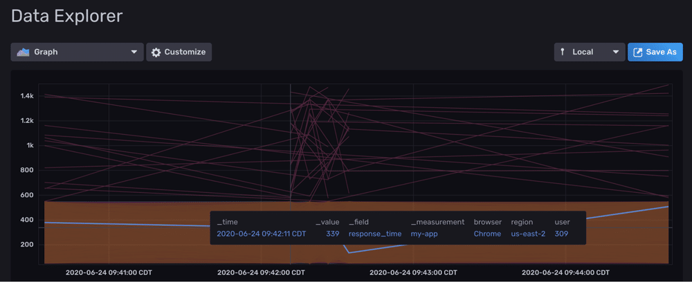
Now that we’re convinced that the MAD function is pretty sensitive to anomalies, let’s take a look at its performance on large datasets. For this example, we’ll imagine that we’re monitoring response times for a web application. We’ve been collecting event data that contains the response time for various users. Tags describe the users’ region and browser. We have around  90k points in the following window.

We then apply MAD with the following script which only took 6s to execute on my local machine with other processes running. In this example, I import the package after compiling Flux. Once the Pull Request is merged, you should be able to apply MAD like this:

import "contrib/anaisdg/anomalydetection"

mydata = from(bucket: "my-app-response")
  |> range(start: v.timeRangeStart, stop: v.timeRangeStop)
  |> filter(fn: (r) => r["_measurement"] == "my-app")
  |> filter(fn: (r) => r["_field"] == "response_time")

mydata |>anomalydetection.mad(threshold:3.0)
             |> filter(fn: (r) => r.level == "anomaly")

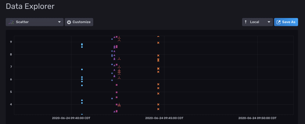
We can see that we have quite a few response times that are above 500 ms. Now we can identify what might be causing these slow response times by analyzing the anomalies. After grouping by region and counting the values with:

mydata |> mad(threshold:3.0)
       |> filter(fn: (r) => r.level == "anomaly")
       |> group(columns: ["region"])
       |> count()

We arrive at some conclusions. Users that use IE6 have slower response times, and there might be some issue occurring in the us-east-2 region, as most of the anomalies are occurring there.

A kind request and conclusion

In this post, we learned how we can use Flux to write simple but powerful anomaly detection algorithms. We learned that it is both fairly sensitive and efficient. However, I’d be remiss if I didn’t outline the subsequent natural steps and additional tools to take advantage of.

To complete a an anomaly detection pipeline in InfluxDB 2.0 and Flux:

1. Write a Task to write these anomalies to a new bucket using the to() function.
2. Alert on the anomalies.
3. Take advantage of the http.post() function to trigger a script and automate corrective action in response to the alert.

Important Note: Since this function performs calculations that are grouped by time, you could create a task that runs the MAD function frequently – you could attempt to mirror the data collection frequency/interval rather than waiting to run this over a longer time horizon. Executing the MAD function more frequently decreases the input data and increases performance to accommodate even larger datasets. 

One thing that makes Flux and InfluxDB stack special and powerful is that they are open source. InfluxDB and Telegraf wouldn’t be where they are today without help from the community. Flux, although already extremely powerful in beta, can use your help too. The MAD function here from the anaisdg/anomalydetection Flux package is special because it was contributed as a Third Party Flux Package. If you’ve written custom Flux Functions to perform anomaly detection or other forecasting, I encourage you to contribute them. Let others benefit from your hard work and sing your praises!

To learn more about contributing Third Party Flux Packages, please read this blog. As always, please share your thoughts, concerns, or questions in the comments section, on our community site, or in our Slack channel. We’d love to get your feedback and help you with any problems you run into! Again, thank you!